$MobileNet$ 系列算法之 $V2$
针对 $MobileNet$-$V1$ 中出现的 $Depthwise$ 部分的卷积核容易废掉,即卷积核参数大部分为零的问题,$Google$ 团队在 $2018$ 年提出 $MobileNet$-$V2$,相比于 $MobileNet$-$V1$ 网络,准确率更高,模型更小。
简介
主要有以下两个亮点:
使用了 $Inverted$ $Residuals$(倒残差结构)
使用了 $Linear$ $Bottlenecks$
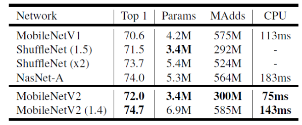
如下图 1 所示为 $MobileNet$-$V2$ 和其他网络的一些性能对比。从图可知, $MobileNet$-$V2$ 相比于 $MobileNet$-$V1$ 性能提升了 $1.4$ 个点,并且参数量和计算量都降低了很多,单图推理性能达到 $75ms$。甚至于采用 α(在 $MobileNet$-$V1$ 中的宽度因子)=$1.4$ 的情况下,精确度上升至 $74.7$。
$Inverted$ $Residuals$
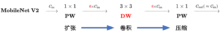
在 $MobileNet$-$V1$ 中的 $DW$ 深度卷积本身没有改变通道数量的能力,输入通道数等于输出通道数。如果来的通道很少的话,$DW$ 深度卷积只能在低维度上工作,这样效果并不会很好,所以作者提出要“扩张”通道。既然已经知道 $PW$ 逐点卷积也就是 $1×1$ 卷积可以用来升维和降维,那就可以在 $DW$ 深度卷积之前使用 $PW$ 卷积进行升维,再在一个更高维的空间中进行卷积操作来提取特征。如下图所示,这种在深度卷积之前扩充通道的操作在 $v2$ 中被称作 $Expansion$ $layer$,如下图 2 所示。
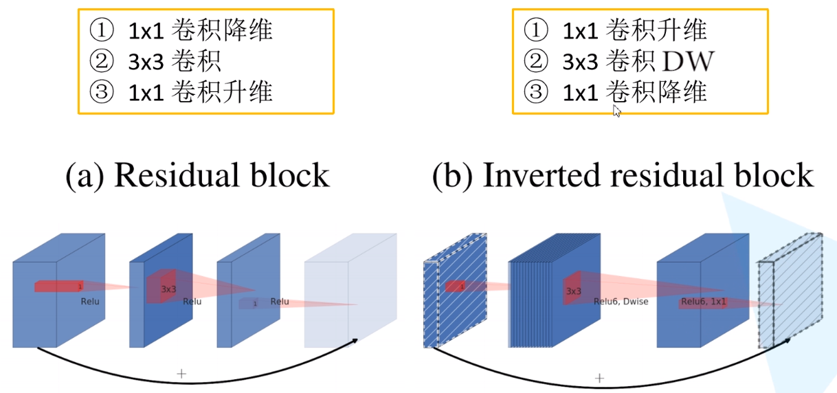
$MobileNet$-$v1$ 虽然加了深度可分离卷积,但网络主体仍然是 $VGG$ 的直筒型结构。而$MobileNet$-$v2$ 网络的另外一个关键点就是借鉴了 $ResNet$ 的残差结构,在 $MobileNet$-$v1$ 网络结构基础上加入了跳跃连接。相较于 $ResNet$ 的残差块结构,作者在 $MobileNet$-$v2$ 中给这种结构命名为 $Inverted$ $resdiual$ $block$,即倒残差块。至于为什么叫倒残差网络是因为,如下图 $3$ 中 $a$ 图所示的传统残差块是先做 $1×1$ 卷积降维再做 $3×3$ 卷积和 $1×1$ 卷积升维的操作,呈现“两头大,中间小”的效果,而 $Inverted$ $resdiual$ 如下图 3 中 $b$ 图所示是先做 $1×1$ 卷积升维再做 $3×3$ 卷积和 $1×1$ 卷积降维,呈现“两头小,中间大”的效果,故而叫做“倒残差”块,之后再做 $shortcuts$ 操作增加跳跃连接,目的是为了减缓梯度传播时造成的梯度弥散。
$Linear$ $Bottlenecks$
在 $MobileNet$-$V1$ 中会出现 $Depthwise$ 部分的卷积核容易废掉,即卷积核参数大部分为零的现象,经过作者的分析之后得出这个问题其实是由于 $ReLU$ 激活函数导致的。
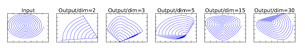
什么意思呢?作者在原论文中也给出了解释,如下图 $4$ 所示为将低维流形的 $ReLU$ 变换 $embedded$ 到高维空间中的例子,用比较通俗的话来讲就是将一个 $n$ 维的特征 $T$ 做 $ReLU$ 运算,然后利用 $T$ 的逆矩阵进行恢复,从图 $4$ 中可以看出,当 $n = 2,3$ 时,恢复出现的特征与 $Input$ 相比有很大一部分的信息已经丢失了。而当 $n$ = $15$ 到 $30$,还是有相当多的地方被保留了下来。也就是说,对低维度做 $ReLU$ 运算,很容易造成信息的丢失。而在高维度进行 $ReLU$ 运算的话,信息的丢失则会很少。
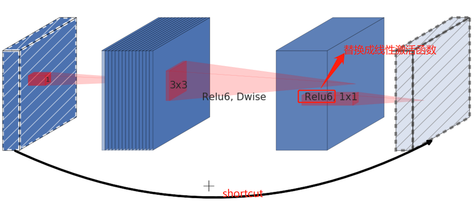
这就解释了为什么深度卷积的卷积核有不少值是空的。而作者给出的解决方案就是:既然是 $ReLU$ 导致的信息损耗,将 $ReLU$ 替换成线性激活函数,当然了并不是将所有的 $ReLU$ 函数都替换为线性激活函数,而是将 $Inverted$ $Residuals$(倒残差结构)中的最后一个 $Relu6$ 激活函数换成线性激活函数,如下图 $5$ 中所示,将红色框中的 $ReLU6$ 替换成线性激活函数。
整体结构
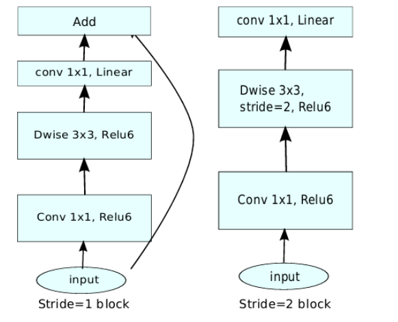
作者在采用了以上两种方式的改进后,最终的 $MobileNet$-$V2$ 的两种 $Inverted$ $Residuals$ $bottleneck$ 如下图 $6$ 所示,需要注意的时候,只有在 $stride$=$1$ 并且输入特征 $shape$ 和输入特征 $shape$ 一致的情况下才加入 $shortcuts$ 操作。如果是 $stride$=2 的话,则采用的是下图中右边的 $Inverted$ $Residuals$ $bottleneck$。
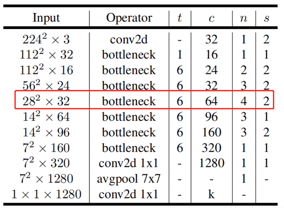
如下图所示为 $MobileNet$-$V2$ 的整体网络结构,在图中 $n$ 代表 $bottleneck$ 的重复次数,$s$ 代表步长,$c$ 代表输出维度。需要注意的是,在每一个重复的 $bottleneck$ 中只有第一层的 $bottleneck$ 的 $stride$ 为 $s$,其他的为 $1$,例如在 $28×28×32$ 的 $bottleneck$ 重复了四次,只有第一次的 $bottleneck$ 的 $stride$ 为 $2$,其余的为 $1$,原因是因为第一次的 $bottleneck$ 的 $stride$ 为 $2$,输入和输入的 $shape$ 不一样,因此采用的是上图 $6$ 中的右边的 $bottleneck$,而剩下的 $bottleneck$ 的 $stride$ 为 $1$,输入和输出 $shape$ 是一致的,采用的是上图 $6$ 中的左边的 $bottleneck$。
核心代码如下所示:
总结
1、$MobileNet$-$V2$ 提出了 $ReLU$ 激活函数会丢失低纬度的信息,因此采用了 $Linear$ $Bottlenecks$,取得了很好的效果。
2、借鉴了 $Resnet$ 的思想,提出 $Inverted$ $Residuals$(倒残差结构)。
3、基于以上两点的改进,$MobileNet$-$V2$ 比 $MobileNet$-$V1$ 精度更高,计算量和参数量也更少。
引用
https://arxiv.org/pdf/1801.04381.pdf
https://zhuanlan.zhihu.com/p/58217659
https://www.cnblogs.com/wxkang/p/14128415.html
https://blog.csdn.net/liuxiaoheng1992/article/details/103602929
https://mp.weixin.qq.com/s?src=11×tamp=1622358786&ver=3099&signature=tbckX3Ag4sZl23EHKVEwpMiWWZs5YCLJsEuMNnewpUqT1JPMMVHPeva8FzQuBGjT7bHg0X-he3eKs0AT22iwsQ58V02sQJpzm-aCxSMj54AYuKbEqAp*EASUAkCPLEGH&new=1
https://blog.csdn.net/weixin_44023658/article/details/105962635?utm_medium=distribute.pc_relevant.none-task-blog-baidujs_title-0&spm=1001.2101.3001.4242
Last updated